| Chapter 5. Presenting Input to the Program | ||
|---|---|---|

|
Part I. AMPAC™ 10 User Guide |  |
| Chapter 5. Presenting Input to the Program | ||
|---|---|---|
|
|
Part I. AMPAC™ 10 User Guide | |
Abstract
The structure and components of an AMPAC™ data file will be
discussed in this chapter. The AMPAC input file is simple in
structure and has several required sections along with a number of optional sections for
specialized tasks. All data are passed to the program via the data file
(jobname.datjobname.outjobname.arc
Table of Contents
|
Section 1: |
Keywords (one or more lines) |
|
Section 2: |
Title (one line required) |
|
Section 3: |
Comments (one line required) |
|
Section 4: |
Geometry Specification (multiple lines terminated by one blank line or all zeros) |
|
Section 5: |
CHN/CHAIN Geometries (one or more additional z-matrices separated by and terminated by one blank line or all zeros) |
|
Section 6: |
Extra Input Data (symmetry, reaction path data, etc.) |
Keywords are the communication link between the user and AMPAC. The type and method of calculation is defined by selecting the proper set of keywords (see Chapter 6, Keywords for a full description of each keyword). Keywords may be arranged in any order, may be upper or lower case (or mixed), but must be separated from one another by at least one blank space. Note that some keywords require additional data to be added at the bottom of the input file (Section 6 in the above list). {In the GUI, most keywords are accessible via the AMPAC Dialog Box or special purpose subdialogs. Those that cannot be activated in this fashion are accessible through the GUI by placing them on the “additional keywords” line in the main AMPAC dialog box. Note that any unrecognized keywords will be placed on this line when a results file is read into the GUI.}
AMPAC allows the keyword line to extend over multiple lines such that the total number of characters is less than 500. The program looks for additional keyword lines if the last characters on the line are a blank and a plus sign: “+”. The following is an example of a multiple-line keyword definition:
 am1 rhf singlet t=auto truste gradients +
sc.i.=4 noxyz cistate=2 +
meci bonds ci-ok
“Title”
“Comments”
Some keywords should be present in almost every AMPAC input deck. We recommend the following:
am1 truste gradients bonds t=auto
The first keyword, AM1, specifies the particular semiempirical method to be used. For purposes of clarity and consistency, this should always be the first item on any keyword line. As noted above, the MINDO3, MNDO, MNDO-d, PM3, MNDOC, SAM1, and AM1 methods are available in AMPAC, but for general purpose use we favor the highly successful and extensively tested AM1 procedure. However, there is no default method in AMPAC; a method keyword must be specified or the job will fail.
AMPAC includes a filter for testing for allowed MINDO3 atom pairs upon input. Note that even a non-bonded atom pair for which there are no parameters is not permitted by this check. The reason for this is that there is no adequate rule for determining a distance cutoff in this context. For most situations (except perhaps cations) one of the NDDO methods such as AM1 or SAM1 is preferable to MINDO3.
TRUSTE specifies what type of job that AMPAC is to perform. This keyword tells AMPAC to optimize the geometry by minimizing the energy (heat of formation) of the molecule. If no job type is specified then AMPAC will perform a TRUSTE optimization by default.
The keyword GRADIENTS forces reporting of the final normalized gradient (“gnorm”) and the components of the gnorm corresponding to each optimizable geometric parameter resulting from the geometry optimization. It also provides a listing of each geometric parameter’s contribution to the gnorm. At an optimized geometry, the overall gnorm should be close to zero, as should the value for each component. Generally, a gnorm value of less than 1.00 indicates a successful geometry search. In the cases of very large molecules, however, this number may be larger than 1.00 due to the sheer number of contributors. See the section called “Calculation of Gradient Norms” for a discussion of computation of the gnorm.
The BONDS keyword prints the non-zero elements of final two-center bond order matrix. This information should directly correspond to the valence bond picture of the molecule, {and is used by the GUI to draw bonds on screen. In the absence of such information the GUI uses an interatomic distance alogorithm to draw bonds.}
T=AUTO tells AMPAC to automatically determine how much CPU time is to be allowed for the calculation. If the calculation is expected to exceed its allocated time, the calculation will stop and restart files will be written. This is done to ensure that long jobs may be restarted while also guarding against runaway jobs. Generally, T=AUTO will allocate 1 hour of CPU time for the calculation but is more flexible than T=1H in that for certain job types (such as CHN and ANNEAL), AMPAC may automatically choose a larger time limit if deemed necessary.
The first line after the keyword line is the title line and the immediate next line is the comment line. Both lines must be present (although they may be blank) even if the user does not wish to fill in any information because the program expects there to be text in this position. Based on common usage, it is suggested that the title line should contain the name and chemical formula of the compound and the comment line contain information about the person performing the calculation, date, and other relevant items. However, any information may be placed on either line, as they are simply text fields.
The spatial arrangement of the nuclei of a molecule can be specified either by Cartesian or internal coordinates. Internal coordinates are convenient in that they represent chemically intuitive items that can usually be estimated a priori and have meaning a posteriori. Cartesian coordinates are available from many sources and also define an absolute orientation for the molecule. The initial coordinates for each atom are used as the starting geometry for further calculation. It must be emphasized at this point, that whichever method is chosen to enter the geometry, atomic positions are all that is being provided to the program. Information about bond connectivity, such as would be found in a molecular mechanics input file, is not required in AMPAC. Based on the results of the electronic structure calculation, bonding is determined instead from the wavefunction.
Three internal coordinates for each atom are required (except for atoms 1, 2, and 3, see below). These are arranged in standard z-matrix fashion.[16] The three internal coordinates for the atoms are the bond length, bond angle, and dihedral angle. Each of these items is referenced to other atoms that have already been defined. In some cases, care must be exercised as to the order of atomic definition. AMPAC geometry input lines are “free-format”, that is the items do not need to be in specific columns to be read properly. The items must, however, be presented in the correct order. The standard form for a line of an internal coordinate z-matrix is listed below:
Symbol Bond Length Bond Angle Dihedral Angle NA NB NC Spec
The symbol of an element can be defined by either letters (referencing specific elements on the periodic table) or atomic numbers. Differences between lower case and upper case characters are ignored.
When an element symbol is used by itself, the element’s standard atomic mass will be used in the calculation. This is what is desired in most cases but sometimes it is necessary to specify particular masses to be used in the calculation, e.g. kinetic isotope effect or vibrational frequency studies. To use the mass of a specific isotope, the number of the isotope is placed directly after the corresponding atomic symbol, with no spaces. Thus for carbon-13:
C13 1.54 1 109.50 1 180.00 1 3 2 1
If the specific isotope is not recognized by Ampac or a particular mass is needed, simply place the number after the atomic symbol (with no spaces). (To distinguish a user-specified mass from an isotope, it must contain a decimal point.) As an example, to give a carbon atom a mass of 13.005:
C13.005 1.54 1 109.50 1 180.00 1 3 2 1
Both modes of specifying the mass for an atom apply to Cartesian coordinates as well.
The optimization flags (BL, BA, and DA) are listed for the
preceding geometric variable. If a flag is set to zero, the variable
is not optimized in the course of the calculation. If the value is set to one, the parameter
is allowed to vary. Definitions of reaction coordinates and grid search patterns can also be
specified by way of the optimization flags (see Chapter 25, One-Dimensional Reaction Pathway,
Chapter 26, Two-Dimensional Grid Search and the keyword pair
STEP1=n.n,
STEP2=m.m).
NA, NB, and NC are the
numbers of previously defined atoms to which the geometric parameters of the present atom are referenced.
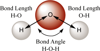
The bond length of an atom is with reference to one other atom, and is the distance from that atom in Angstroms. The value for a bond length must be greater than zero. In the case of the AMPAC input line, the bond length is referenced to atom NA. While the term “bond length”[17] is used, a better descriptor might be “interatomic distance”. For purposes of geometry definition, the atoms are not required to be chemically bonded either at the beginning or end of the calculation. The structure of a molecule is usually defined, however, by the bonding framework. This is easier to conceptualize and standard values for bond lengths are available in tabular form from a number of convenient sources.[18] If atoms are defined via the bonding network, this also makes the interpretation of the output easier as these chemically important values are direct results of the calculation. Note that the first atom in a z-matrix does not have a bond length, as there is no preceding atom from which to reference the bond length. The second and all succeeding atoms have bond length values.
The bond angle[19] of an atom is with reference to two other atoms and is simply the angle formed by the three atoms (See Figure 5.1, “Bond Lengths and Bond Angle for Water”). The values for bonds angles must be positive. In the protocol of AMPAC, this is the angle XNANB (where X is the present atom). Note again that it is not required that the atoms used to define a bond angle be chemically connected to one another. It is not possible to define a bond angle until atom number three is listed. Thus atom 3 and all subsequent atoms have bond angles. AMPAC requires all bond angles to be positive.
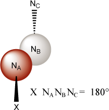
The dihedral angle (also referred to as the torsional or tortional angle in some cases) is defined by reference to three previously defined atoms. The dihedral is defined as the angle of rotation about the NANB axis (viewed in this manner) that is required to bring the atom under consideration (X) into alignment with atom NC. (See Figure 5.2, “Newman Projection Showing Dihedral Angle Definition”) Dihedrals may either be positive or negative. The possible range is -360 to +360, although AMPAC will translate all dihedrals to -180 to +180. (Thus an input dihedral value of 240 will be output as -120.) It is required that the three atoms to which the dihedral of a fourth atom is referenced do not assume a straight line arrangement either as a part of the definition or as a result of the geometry optimization. The program checks for this condition at the beginning of the input and also at each step in the geometry optimization. This difficulty (e.g. encountered in the definition of alkynes) can be circumvented by the use of dummy atoms.
The sign convention for defining dihedral angles in AMPAC is as follows:
When looking down the NA-NB axis, the dihedral angle is positive if X can be rotated into congruence with NC by moving clockwise less that 180. Conversely, the dihedral angle is negative if X can be rotated into congruence with NC by moving counterclockwise less that 180.
Some examples of dihedral angle definitions are shown below. A dihedral angle cannot be specified until atom number four. All subsequent atoms have dihedrals.
Figure 5.3. Examples of dihedral angle definitions: Methanol

O   0.00  0    0.00  0    0.00  0  0  0  0
C   1.51  1    0.00  0    0.00  0  1  0  0
H   1.00  1  109.50  1    0.00  0  1  2  0
H   1.00  1  109.50  1    0.00  1  2  1  3
H   1.00  1  109.50  1  120.00  1  2  1  4
H   1.00  1  109.50  1 -120.00  1  2  1  4
Figure 5.4. Examples of dihedral angle definitions: Ethene

C   0.00  0    0.00  0    0.00  0  0  0  0
C   1.30  1    0.00  0    0.00  0  1  0  0
H   1.00  1  120.00  1    0.00  0  1  2  0
H   1.00  1  120.00  1  180.00  1  1  2  3
H   1.00  1  120.00  1    0.00  1  2  1  3
H   1.00  1  120.00  1  180.00  1  2  1  5
The above examples illustrate some important principles for defining z-matrices and especially dihedral angles. First, there are several possible schemes that would properly define the geometry of either of these molecules. One advantage the scheme used possesses is that all components of the geometry specification correspond to actual internal coordinates of the molecule: bond lengths define actual bonds and so forth. While it is not always possible to implement this pattern, it is usually simplest.
Another advantage is the “modularity” of the hydrogen atom definitions. In both cases, some of the hydrogen atom dihedral angles are defined with respect to previously defined hydrogens. This allows easy rotation of both species about interatomic axes. For instance in the first example, the entire methyl group could be rotated by simply changing the dihedral of the first hydrogen. The other two hydrogens will “follow” as this one is rotated. Similarly, twist-ethylene could be produced in the second case by changing the dihedral angle of hydrogen 5 to 90 rather than 0. This type of organization is quite useful when a conformational search is being performed or a methyl rotation is interfering with location of a transition state. It is also generally useful to keep functional groups such as phenyls modularized. This allows relatively easy replacement for studies of substituent effects.
As noted above, it is not always possible to use “natural” bond patterns to define a molecule. A classic example is acetylene, C2H2. The first three atoms are easily defined:
C  0.00  0    0.00  0     0.00  0    0  0  0
C  1.20  1    0.00  0     0.00  0    1  0  0
H  1.10  1  180.00  1     0.00  0    1  2  0
There is some difficulty in defining the dihedral of the fourth atom. This atom may not be referenced to the previous three atoms because they fall on a straight line. This will cause the dihedral of the fourth hydrogen to become undefined and the program will generate an error message and halt computation.
The solution to this problem lies in adding “dummy atoms.” These atoms are place holders that have no chemical significance. They simply provide a point in space to which other atoms may be referred, and are commonly applied in the case of linear molecules as noted above. The AMPAC symbol for dummy atoms is “XX” or “Xx”, or they may be specified by the atomic number “99”. Continuing with the example of acetylene, the geometry is redefined below using two dummy atoms. (Note that the dummy atom geometric parameters are not optimized, as they have no chemical significance in this case.)
Figure 5.5. A z-matrix for acetylene using dummy atoms

C   0.00  0    0.00  0     0.00  0    0  0  0
C   1.20  1    0.00  0     0.00  0    1  0  0
XX  1.00  0   90.00  0     0.00  0    1  2  0
XX  1.00  0   90.00  0   180.00  0    2  1  3
H   1.10  1   90.00  1   180.00  1    1  3  2
H   1.10  1   90.00  1   180.00  1    2  4  1
Another use of dummy atoms is for the definition of molecules with particular difficulties. A convenient example is a cyclic ring system such as benzene. (The AMPAC optimization routines handle the case of benzene with no difficulty, but it can be used to illustrate the point for other systems of similar types.) If the carbon skeleton of benzene or some other cyclic system is defined before the hydrogens, a C-C bond is left undefined (i.e. “dangling”):
Figure 5.6. A z-matrix for benzene

C  0.00  0    0.00  0     0.00  0    0  0  0
C  1.40  1    0.00  0     0.00  0    1  0  0
C  1.40  1  120.00  1     0.00  0    1  2  0
C  1.40  1  120.00  1     0.00  1    3  2  1
C  1.40  1  120.00  1     0.00  1    4  3  2
C  1.40  1  120.00  1     0.00  1    5  4  3
Notice that the C1-C6 bond is not specifically defined in this z-matrix. In those cases where an optimization might fail, the problem usually arises when the first geometry optimization step causes a widening of the ring angles because there is no optimizable parameter “closing” the ring. Dummy atoms can be used to solve this case by “spinning” the atoms out from a central position like the spokes on a wheel. This eliminates all explicit bond specifications and the optimization will be more likely to proceed smoothly. Below is an example of the carbon skeleton of benzene defined using a central dummy atom:
Figure 5.7. A z-matrix for benzene using a dummy atom

XX   0.00  0    0.00  0     0.00  0    0  0  0
C    1.40  1    0.00  0     0.00  0    1  0  0
C    1.40  1   60.00  1     0.00  0    1  2  0
C    1.40  1   60.00  1   180.00  1    1  3  2
C    1.40  1   60.00  1   180.00  1    1  4  3
C    1.40  1   60.00  1   180.00  1    1  5  4
C    1.40  1   60.00  1   180.00  1    1  6  5
Some care should be used in employing dummy atoms. In the examples above, the coordinates of the dummy atoms are not optimized. This insures that only the 3N-6 independent internal coordinates (N is the number of atoms) of the molecules are correctly described. If more than 3N-6 parameters are allowed to vary, dependencies will be present during the geometry optimizations which can produce spurious results. For this reason, optimization of dummy atom parameters should not be carried out except in special circumstances. As a general rule, dummy atoms can cause unexpected difficulties in the geometry optimization procedures and should be avoided when possible.
The “Spec” item is used presently for entering partial charges for sparkles.
As well as internal coordinates, Cartesian coordinates (x, y, z) may be used for specification of geometries for AMPAC. This option allows easy interface with other modeling or graphics packages that provide or require the coordinates of atoms in Cartesian space. Each atom is defined by distances along three orthogonal axes and no connectivity list is provided. Following each coordinate is an optimization flag for the preceding coordinate. Note immediately that this type of geometry results in six more parameters to be optimized during the geometry search than an equivalent internal coordinate definition. Although generally of little consequence, this type of definition does require more calculation time than a z-matrix definition scheme. When reading a geometry from an input file, AMPAC will search for a connectivity list at the end of each line. If one is not located, AMPAC will assume that the geometry is in Cartesian coordinates and proceed with input on that basis.
There are several special rules that apply when input is provided in Cartesian coordinates. Unlike previous versions of AMPAC, users may now define optimization options for Cartesian coordinates. Also, the user should be aware that only internal coordinates are used for triatomic systems. (On input, AMPAC assumes a connectivity pattern for the first three atoms, and thus will not allow Cartesian coordinate to be utilized.) The keyword XYZ is not required to define a Cartesian geometry. Its use causes the entire calculation to be performed in Cartesian space, regardless of the initial geometry definition (internal or Cartesian space). (See the discussion of the XYZ keyword.) This is useful in eliminating possible problems with undefined dihedrals during optimizations or searches for transition states, such as might be the case with CHN. It is not necessary to use dummy atoms with Cartesian coordinate definitions.
Four extra “elements” are included in AMPAC. These items represent pure ionic charges, roughly equivalent to the following chemical entities:
Table 5.2. Sparkles
| Symbol | Atomic # | Equivalent to: |
|---|---|---|
| + | 104 | Tetramethyl ammonium radical, K atom or Cs atom. |
| ++ | 103 | Ba atom. |
| - | 106 | Borohydride radical, Halogen, or Nitrate radical. |
| -- | 105 | Sulfate, oxalate. |
For the purposes of discussion these entities are called “sparkles”. They
all have an ionic radius of 0.7 Å so that any two sparkles of opposite sign will form an ion
pair with an interatomic separation of 1.4 Å. They have a zero heat of atomization, no
orbitals, and no ionization potential. They do not contribute to the orbital count, and
cannot accept or donate electrons. Since they appear as uncharged species which immediately
ionize, attention should be given to the charge on the whole system (see the CHARGE=n
keyword). For example: the alkaline metal salt of formic acid would have the formula
HCOO+, where + is the unipositive sparkle. The charge on the
system would then be zero. A water molecule polarized by a positive sparkle would have the
formula H2O+, and the charge on the system
would be +1. A sparkle is best conceptualized as a sphere of diameter 1.4 Å with the charge
delocalized over its surface. Computationally, a sparkle is an integer charge at the center
of a repulsion sphere of form e-αr. The hardness of the sphere
defined by this function is such that other atoms or sparkles can approach within about 2 Å
quite easily, but only with great difficulty come closer than 1.4 Å.
Sparkles find utility in several situations. They can be used as counterions, e.g. for acid anions or for cations. They can also operate as polarization functions. A controlled, shaped electric field can be produced by combining one or more sparkles.
Sparkles may also now be specified with partial charges. This allows the user to construct electrostatic environments of any shape with exactly specified charges at precise locations. This approach may be useful in studying the interaction of a molecule with a simulated active site or receptor region. The partial charges for each sparkle are specified by using one of the four symbols given above and adding a field at the end of the line in the input file. (The field is labeled “Spec” above). The number in this field becomes the sparkle’s new charge. Note that charge accounting within AMPAC still relies on the actual symbols, not the assigned partial charge values. Sparkles may be assigned partial charge values from -20 to +20.
Sparkles can also be used in frequency calculations, but a mass must be provided in the form noted at the beginning of this section for isotopic mass specification (i.e. the symbol followed by the mass with no space between). If no mass is specified for a sparkle, a mass of 10,000 amu is used.
[Only active if CHN, CHECKCHN, or FULLCHN has been specified on the keyword line.] One or more additional z-matrices must be provided if the CHN algorithm is to be called using one of the above keywords. The first geometry in Section 3 of the input file is the initial (reactant) geometry for the reaction path. At least one more z-matrix must follow, each separated from the previous by a blank line or a line of zeros. The final z-matrix is taken to be the final (product) geometry for the reaction path. Any z-matrices between the initial and final geometries will be used to define additional points along the initial reaction path, prior to refinement by the CHN algorithm. See Chapter 8, CHN Methods for a more complete discussion of the CHN algorithm.
[Only active if CHAIN has been specified on the keyword line.] Z-matrices for left and right minima (respectively) must be provided if the CHAIN algorithm is to be used. These are in addition to the first geometry in Section 3 of the input file, which is the “guess” geometry for the transition state used to define the reaction path. The two minima must be separated by a blank line or a line of zeros.
Certain keywords (SYMMETRY, T.V., WEIGHT, LIMIT, and RECLAS) and certain job types (Reaction Paths) require additional data that is not included in the keyword line. This extra input (Section 6) is located immediately following the geometry specification sections (Sections 4 and 5). Starting with AMPAC 8, each extra input section is to be delimited by special section markers (beginning with “$$”). Each data section is then defined as beginning immediately after its unique section marker and ending with the next section marker or the end of the file. When the section markers are used, the data sections may be specified in any order. (For old files and files not using the new section markers, data must be given in a specific order. See the section called “Extra Input Data Using Old Format”.) Section markers are case insensitive and may be abbreviated as specified. A list of recognized section markers is given below.
Table 5.3. Section Markers for Extra Input Data
| Keyword or Job Type | Section Marker | Abbreviation |
|---|---|---|
| SYMMETRY | $$ symmetry - constraints | $$ symm |
| T.V. | $$ t.v. - transition vector coordinates | $$ t.v. |
| WEIGHT | $$ weight - transition vector weights | $$ weig |
| PEN2GRP | $$ pen2grp - pen2 group assignments | $$ pen2grp |
| LIMIT | $$ limit - annealing boundaries | $$ limit |
| RECLAS | $$ reclas - ci permutation of mos | $$ reclas |
| Reaction Paths | $$ rxnpath - values along reaction path | $$ rxnpath |
| [any job type] | $$ properties - external molecular property data | $$ prop |
| [any job type] | $$ connectivity - input connectivity data | $$ connect |
| {end of extra input} | $$ end of extra data | $$ end |
[Only active if SYMMETRY is on the keyword line.] “Symmetry” as used in AMPAC is different than what most chemists think of as symmetry. In the case of geometry definitions for AMPAC, symmetry is used to set certain geometric parameters equal to one another during the course of a geometry optimization. This accomplishes two major objectives. First, the number of variables is decreased and the optimization proceeds more rapidly. Second, AMPAC’s symmetry option allows the user to impose specific constraints on the molecule in keeping with that molecule’s point group or some item of chemical interest. However, caution must be exercised in that imposition of symmetry is a chemical presupposition that may or may not be correct in the context of the problem. If a molecule should be symmetric (is a member of a particular point group), use of the proper symmetry will usually lead to a slightly lower energy than a full optimization where all independent coordinates are varied.
The symmetry utilities are invoked by using the keyword SYMMETRY and then providing a list of functions and relationships in the appropriate place in the input file. AMPAC presently accepts 20 different symmetry functions (see the SYMMETRY keyword description). These functions allow the internal (or Cartesian) coordinates of a molecule to be equated to one another, and in the case of dihedral angles can be defined as the negative of one another, or varied as sums and differences with respect to a reference angle. The method of symmetry definition is a series of lines at the end of the geometry specification section that is interpreted by the program if the SYMMETRY keyword is used. Each line of symmetry information has the following format:
Reference Atom (separator) Symmetry Function (separator) Dependent Atom(s)
In this arrangement, the Reference Atom is the atom whose geometric parameter is used as the beginning value and will be adjusted in the course of the calculation. Symmetry Function is the AMPAC defined symmetry function relating the reference and dependent atoms. The Dependent Atom(s) is one or more atoms to which the indicated symmetry function is applied. The separator can be either a blank space, a tab, or a comma.
The full list of available symmetry relations is as follows:
Table 5.4. Symmetry Functions
| Function | Coordinate | Description |
|---|---|---|
| 1 | Bond Length | is set equal to the reference bond length. |
| 2 | Bond Angle | is set equal to the reference bond angle. |
| 3 | Dihedral Angle | is set equal to the reference dihedral angle. |
| 4 | Dihedral Angle | varies as 90 degrees minus reference dihedral. |
| 5 | Dihedral Angle | varies as 90 degrees plus reference dihedral. |
| 6 | Dihedral Angle | varies as 120 degrees minus reference dihedral. |
| 7 | Dihedral Angle | varies as 120 degrees plus reference dihedral. |
| 8 | Dihedral Angle | varies as 180 degrees minus reference dihedral. |
| 9 | Dihedral Angle | varies as 180 degrees plus reference dihedral. |
| 10 | Dihedral Angle | varies as 240 degrees minus reference dihedral. |
| 11 | Dihedral Angle | varies as 240 degrees plus reference dihedral. |
| 12 | Dihedral Angle | varies as 270 degrees minus reference dihedral. |
| 13 | Dihedral Angle | varies as 270 degrees plus reference dihedral. |
| 14 | Dihedral Angle | varies as the negative of the reference dihedral. |
| 15 | Bond Length | varies as half the reference bond length. |
| 16 | Bond Angle | varies as half the reference bond angle. |
| 17 | Bond Angle | varies as 180 degrees minus reference bond angle. |
| 18 | No Longer Used | |
| 19 | Cartesian x | is set equal to the negative of the reference atom’s x. |
| 20 | Cartesian y | is set equal to the negative of the reference atom’s y. |
| 21 | Cartesian z | is set equal to the negative of the reference atom’s z. |
An example of a symmetry definition is the case of methane, where all four C-H bonds and all bond angles are treated as equivalent and the dihedral of atom 5 is defined as the negative of the dihedral of atom 4:
  am1 rhf singlet truste gradients bonds t=auto symmetry
Methane in Td symmetry
SYMMETRY
 C   0.000000  0    0.000000  0    0.000000  0    0    0    0
 H   1.100000  1    0.000000  0    0.000000  0    1    0    0
 H   1.100000  0  109.500000  1    0.000000  0    1    2    0
 H   1.100000  0  109.500000  0  120.000000  1    1    2    3
 H   1.100000  0  109.500000  0 -120.000000  0    1    2    3
 0   0.000000  0    0.000000  0    0.000000  0    0    0    0
$$ symmetry - constraints
  2,   1,     3, 4,  5
  3,   2,     4, 5
  4,  14,     5
$$ end of extra data
[Only active if the keyword WEIGHT is present along with PATH
and
T.V.] This section is used to provide
weights to particular components of the oriented transition vector supplied for PATH. See
the section called “Input File (irc/path_tv_weight.dat):” for an example of the use of
WEIGHT.
[Only active if the keyword T.V. (but
not T.V.=n) has been specified with either
PATH or
IRC.] This section is used to list the
components of the oriented transition vector for the PATH (in internal coordinates) or IRC
(in Cartesian coordinates) method to follow. See
the section called “Input File (irc/irc.dat):” and the section called “Input File (irc/path_tv_weight.dat):”
for examples of its application.
[Only active if one of ANNEAL, MANNEAL, GANNEAL or TSANNEAL has been specified along with PEN2GRP.] PEN2GRP is an extension of PEN2 that only applies the penalty for atoms belonging to the same group. Information defining the atomic groupings is read in here in the extra input section. The data must contain a list of positive integers, one for each atom in the molecule, in free format. The nth integer represents fragment group to which the nth atom is to be assigned. The group number may range from 1 to the total number of atoms. This input can be further simplified by grouping consecutive identical indices using the “n*m” abbreviation. For example, a sequence of 10 atoms all belonging to group 2 can be abbreviated as “10*2”. See Chapter 13, Simulated Annealing for a detailed explanation on the use of simulated annealing keywords.
[Only active if one of ANNEAL, MANNEAL, GANNEAL or TSANNEAL has been specified along with LIMIT.] This section is used to provide upper and lower bounds for each optimizable geometric parameter in the annealing procedure. The lower bound for each parameter is given first (in free format, up to 80 characters per line, in order of appearance on the z-matrix) and next the upper bound for each parameter in the same order and fashion as the lower bound). See Chapter 13, Simulated Annealing for a detailed explanation on the use of simulated annealing keywords.
[Only active if C.I.(n,m) is specified and RECLAS is also used.] This section
describes the perturbation of MOs for use in the CI procedure. See Chapter 11, Configuration Interaction for a discussion of the use of RECLAS.
[Only active for reaction path calculations. The calculation is a reaction path if one of the geometric parameters is marked with a “-1” for the optimization flag.] One of the optimizable geometric parameters may be designated as the “reaction coordinate.” This is typically done in order to locate the position of an approximate transition state along a proposed reaction pathway. The definition is accomplished by marking that item with a -1 as its optimization flag. The values supplied in this section of the input file are then substituted one after another (the first value used is that in the geometry itself) and the requested properties computed at each value. See Chapter 25, One-Dimensional Reaction Pathway for a more complete description of the use of the reaction coordinate.
[Read for all job types.] This section allows the user to supply additional property information about
the molecular system. This information has no effect on the calcuation but is passed through to the
.out, .arc,
and .vis files. However, in the case of multi-geometry
job types (i.e. everything but single point calcuations, optimizations, and frequency jobs), this data
will simply be surpressed. This is because this extra data is connected to the input configureation
and so would not have the same meaning or relevance to output of multi-geomtry jobs.
[Read for all job types.] User-specified information about the connectivity of the input structure can be
specified here. Currently, this is not usued during the calculation but is passed through to the
.out, .arc,
and .vis files. However, in the case of multi-geometry
job types (i.e. everything but single point calcuations, optimizations, and frequency jobs), this data
will simply be surpressed. This is because this extra data is connected to the input configureation
and so would not have the same meaning or relevance to output of multi-geomtry jobs.
AMPAC 10 still supports the old style of extra input data. AMPAC will look first for the extra input section markers and if found will read data from that point in the file. If the specific section marker is missing, then AMPAC will begin reading whatever it finds just after the geometries. Because of this, each extra input section must be in the correct order listed below. If a mixture of the old and new formats is used, then all unmarked sections (old format) should be listed first in the order given below followed by all of the marked sections (new format). The format of the data within each section is the same regardless of whether it is using the old or new format, except that two of them require explicit termination by a blank line or line of zeros.
Symmetry Definitions (multiple lines terminated by one blank line or all zeros)
Reaction Path Coordinates (multiple lines terminated by one blank line or all zeros)
Transition Vector Weights
Transition Vector Specification
PEN2 Group Information
Simulated Annealing LIMIT data
RECLAS Permutation of MOs for CI
The newest extra data sections--external property data and input connectivity--will only be accepted in the new format.
[16] The actual form of the matrix with AMPAC is an x-matrix. That is, the first atom is located at the origin and the first bond is along the x-axis of an orthogonal Cartesian coordinate system. Historically, the first bond was defined to be along the z axis, hence z-matrix. The term z-matrix, while strictly incorrect for AMPAC, has become common usage and will be retained here.
[17] All length measurements in AMPAC are in angstroms (Å), whether Cartesian or internal coordinates are used.
[18] The Chemist’s Companion. John Wiley & Sons. New York . 1972.
[19] All angular measurements in AMPAC are in terms of degrees, whether for bond angles or dihedral angles.
|
Copyright © 1992-2013 Semichem, Inc. All rights reserved. |
|
|
 |
|
| Chapter 4. Computational Procedures |  |
Chapter 6. Keywords |